Today we’ll begin with an interesting and important theorem about the Riemann zeta function. Recall that this is defined when  by the absolutely convergent series

This can be analytically continued to a function meromorphic on the entire complex plane, holomorphic everywhere except for a simple pole at  . Also, we know that it obeys the following functional equation whenever
  :
:

It isn’t hard to show that  whenever
  , and hence the functional equation shows that apart from possible zeros in the critical strip
  the only zeros of
  are the so-called ‘trivial zeroes’ at
  .
.
The functional equation also shows that zeros are symmetrically distributed about the line  . The infamous Riemann hypothesis conjectures that this symmetry collapses so that all non-trivial zeros of occur on the line .
This is a whirlwind summary, and we’ll introduce or elaborate on other properties of as they are needed. It is not trivial that should have any zeros in the critical strip at all, though it actually does. We now know the first  or so zeros, and sure enough, they all lie on the critical line .
It had been shown soon after its introduction that had infinitely many non-trivial zeros. Very little was known about the distribution of these zeros in regards to the critical line was known until 1914 when Hardy proved the following.
Theorem 1 There are infinitely many zeros of on the critical line .
This is a result seemingly more often quoted than proved, and the proof is rather technical and difficult. I have always found it astounding, however, and intrigued by what methods could accomplish this feat. Hence I shall blog the proof of this theorem in a ‘top down’ fashion: first giving the outline of the proof, and then filling in the technical lemmas as needed. I will be following closely the proof given in Montgomery and Vaughan’s “Multiplicative Number Theory” in chapter 14.
Firstly, we note that the function we are really bothered about for this theorem is the function of the real variable  defined by

After all, we’re not going to even attempt to discover anything about away from this critical line. If we can show that this function of has infinitely many zeros, then we’re done. This should be easier for a start, since now we’re only dealing with a function of a real variable rather than a complex variable.
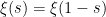
But, unfortunately, this function is not always real-valued itself. Looking back at the functional equation, we can see why — has a fundamentally ‘asymmetric’ nature. To fix this, we recast the functional equation by first defining
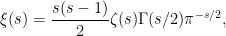
and then noting that after some analytic manipulation the functional equation can be rephrased as
for all  . In particular, since we also have the reflection property
  , we see that this functional equation implies that
  is real for all real . Furthermore, has a zero at
  if and only if
  does.
does.
It suffices, then, to show that the function has infinitely many zeros . This is already much easier to handle, since it is a function from  to . This is nearly the actual function we will consider. However, in some ways remains easier to analyse than
  , and so we’ll normalise so that the absolute value of the function always agrees with that of .
Putting all this together, we can finally define the Hardy  -function as

where the function  is chosen so that
  for all . We can be explicit, looking at the definition of , and define

The function  will change sign
  if and only if
  has a zero at
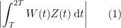
  of odd multiplicity. There is an easy way to detect when a function has a sign change in the interval
 ![{[T,2T]}](https://s0.wp.com/latex.php?latex=%7B%5BT%2C2T%5D%7D&bg=ffffff&fg=000000&s=0&c=20201002) — if and only if the inequality
— if and only if the inequality
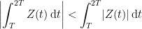
is sharp. If we could show that was true for arbitrarily large  , we’d be done. This is possible, but hard.
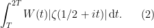
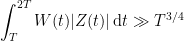
To make things easier, we will first multiply by some suitably chosen kernel  . We’ll make sure that
  for all , so it won’t mess things up. It will hopefully make the analysis simpler.
We’ll choose later. For now, remember that we’ve boiled down the proof to deriving a contradiction from the assumption that for all sufficiently large ,


 (which is just a measurable function
  where
where  is a probability measure space) symmetric if
  . Symmetric random variables are often a lot more pleasant to handle. Much of what is true for symmetric random variables is also true in general, but both the proofs and statements are lot more complicated. For this reason, it would be very useful to know that we can always assume, in some sense, that a random variable is symmetric. This process, finding a related random variable which is symmetric, is known as symmetrization. With a good understanding of this process many proofs in probability become vastly simpler: one can first reduce to the symmetric case, and then just do it by hand.
 , where
  is a random variable identical in distribution to
  , and it is clearly symmetric. Furthermore, note that
  .
. and
and  we have
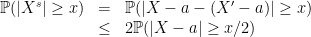
 originally, then
  and real number

 are independent random variables with finite moments of order
  and
and 
 we have
 is identically distributed to
  .
.  , let
, let  be the least
  such that, for all
  sufficiently large (how large can depend on
  such that
 . In other words, past some (possible very large) integer, all integers are the sum of at most some constant number of
  . In fact, we can make the stronger statement that all integers, not just the large ones, are the sum of at most four squares.
 (and hence, in particular,
 will always denote an integer congruent to 1 modulo 6. Define

 — a quick computation shows that this is true for
  , for example. It follows that if we define the interval
 ![{I_z=[\phi(z),\psi(z)]}](https://s0.wp.com/latex.php?latex=%7BI_z%3D%5B%5Cphi%28z%29%2C%5Cpsi%28z%29%5D%7D&bg=ffffff&fg=000000&s=0&c=20201002) then these overlap, and so for
then these overlap, and so for  is in one of these intervals.
 for some fixed
  cubes.
 ,
,  be the smallest positive integers such that


 . Hence
  is a multiple of
  , so we can write
 . If
. If  were some constant, we could stop here having shown that
  , but unfortunately
  . Hence we can write
  . Plugging this into the above and doing some elementary algebra proves the identity
 , so here is where we needed
  by hand, or by being clever first and then checking by hand, it can be shown that in fact every integer is the sum of at most 13 cubes.
  . This can be proved in a way similar to the above if we assumed that every integer which is not of the form
  is actually the sum of three squares. This is true, but difficult.
 elements in arithmetic progression” as part of his proof of what is now known as Szemerèdi’s theorem – a cornerstone of additive combinatorics and one which I’m sure we’ll come back to in a future post.
 and
and  . Define the density
  between
  ). For any parameter
  we say that
  -regular if we have
 and
and  are subsets of
  and
and  .
. such that any graph
  with vertex set
  chunks
  such that the following hold:
 ,
, differ in size by at most one element from one another, and
 of the pairs
  are
are 
 , which controls how many chunks are in this regular decomposition, depends only on
  which is of height roughly
  . Even for fairly large
  if the support of the Fourier transform of
  is entirely contained inside a dissociated set (we’ll come to what that means later) then for any
  we have

 norms over the group
  denote the support of the Fourier transform of
 as
as  instead, indexed over
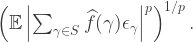
 to a function
  .
. . We will now try to make this heuristic precise, and deduce Rudin’s inequality as a corollary of Khintchine’s inequality. The following follows the proof of Rudin’s inequality given in [Gr1].
 by introducing a random assignment of signs to get
  , where
  are independent random variables taking the values
  . Khintchine’s inequality then gives, for any fixed
  ,
,
 we get (taking
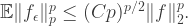
 by
by  . This is useful because it allows us to write
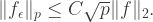
 norm equal to 1. It follows that we can bound
  for any
  and we have proven Rudin’s inequality. Notice that here was where we really needed
  , to pass from a randomised version of
  taking the values
  in any
  norm of the coefficients
  , we have the following bound
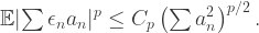
 depends only on
  , and we shall obtain an explicit value below. The inequality is perhaps more suggestive if we observe that
  , where the
 gives
gives
 applying Markov’s inequality and setting
  gives the inequality

 to do the integration, we compute that

 is some absolute constant.
 we also get a similar lower bound.
 of an abelian group, and I told you it was additively structured. There are lots of different things this vague term could mean:
 is not much bigger than
  such that
  (the number of such quadruplets is called the additive energy, and I denote it by
  ).
). , is lumpy and takes on large values quite often.
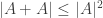 , or
, or  , and so on. In general, we can measure how much better we can do than these trivial bounds, which gives us some parameter which measures how structured our set is. By showing rough equivalence, I mean that if we know that one type of structure is true for some parameter
  (we say that
  let
let  denote the number of pairs
  such that
  . It is easy to see that

 , which means that
  then we get the best possible
  and if
  then we get the trivial
  . We leave it as an exercise for the reader to interpret these facts.
 . In general, we can’t hope for equivalences this strong, and for some any kind of polynomial dependence on